Tangent Plane — An important concept for deriving Gradient Descent
As we know in 2 dimensional space the tangent line is drawn for a parabola. What if we have multi dimensional plane, the tangent line for the parabola in multi dimensional would be obtained by cutting the plane and drawing tangent which would be 2 tangent perpendicular to each other. That is when we can it as tangent plane.
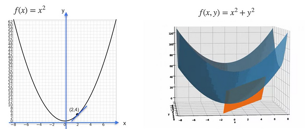
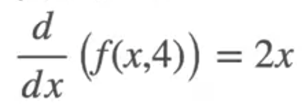
for the equation, f(x , y ) = x² + y² , let us fix the value of y=4 then the equation would be f(x , 4) = x² + 4². The derivative of the f(x) with respect to x would be
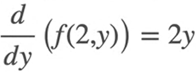
Let us fix the value of x = 2, the equation becomes f(2 , y) = 2² + y², then the derivative of f(y) with respect to y would be
The plot of Tangent plane looks like this
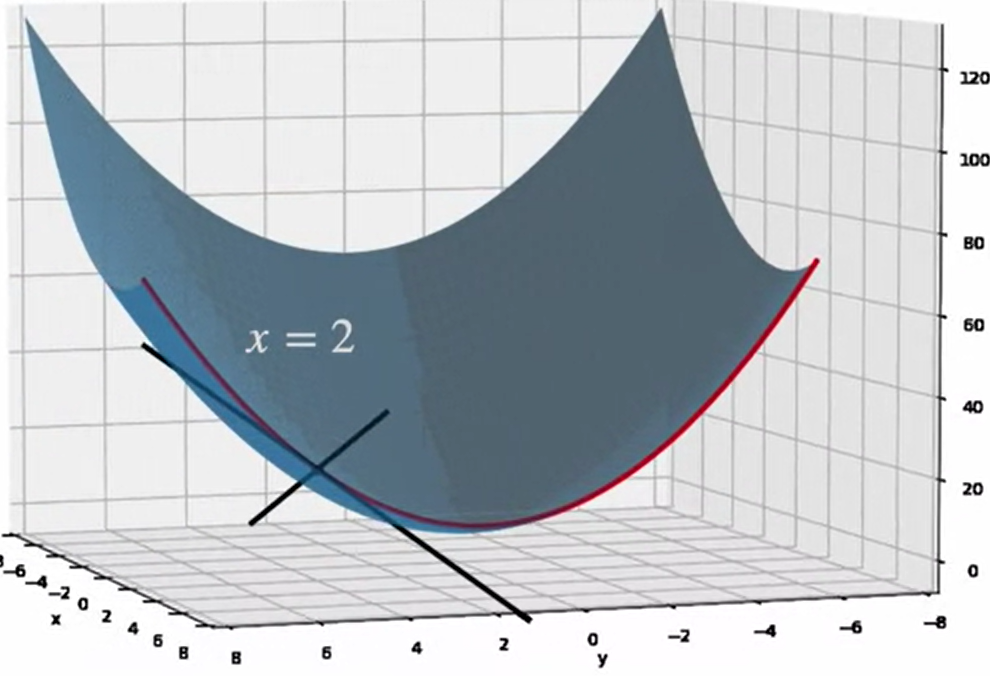
In the above diagram, when we cut the plane you get the red parabola and the red parabola is a function of one variable. So you can draw tangents which is called the Partial Derivative
When we take one variable as a constant as we fixed in the above example, then it becomes a function of one variable and the derivative of the constant would be 0. So the slope in the above case would be 2x if y is taken as constant and 2y if x is taken as constant
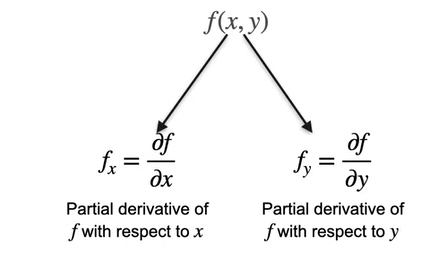
When we are differentiating the equation with respect to 1 variable,
- We treat all other variables as a constant. In our case y.
- Differentiate the function using the normal rules of differentiation.
What is Gradient?
As we have seen in the above example, we treat x as constant in one case and y as constant in other case. The gradient is nothing but the matrix of the derivatives of those 2 values.
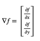
If there are n number of variables, then it would be matrix with n variables.
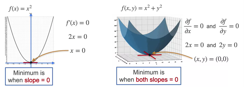
Gradient is used to minimize the error of 2 or more variables.
Same like the tangent line at slope=0 which is the derivative =0 is the minima of the 2 dimensional space, we have Tangent plan at which both the tangent lines are at minima, which is both the partial derivatives are 0.
This is used heavily in the analytical method called Linear Regression.
Our goal is to find the best fit line of the data points and this is found by calculating the line that has minimum sum of squares of error which is difference between the point on the line to the actual data point.
As we have seen above, the partial derivatives can be used to find the optimal point where the error is minimum.
Suppose we have y = mx + b, and substitute the x and y of each data point and find the difference of the datapoint on the line and doing a sum of squares will give something like this.
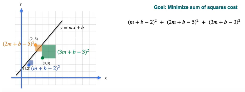
From the above diagram, the cost function that should be minimized is
E(m , b) = 14m² + 3b² +38 +12 mb — 42m — 20b
By applying the partial derivative of the equation with respect to m and then b we get m = 0.5 and b = 7/3
When we substitute in the equation of E we get approximately 4.167 which is the minimum value of the cost.
What if we could not get to the solution of m and b, it is pretty tedious to solve those equations in reality. So Gradient Descent helps in this case.
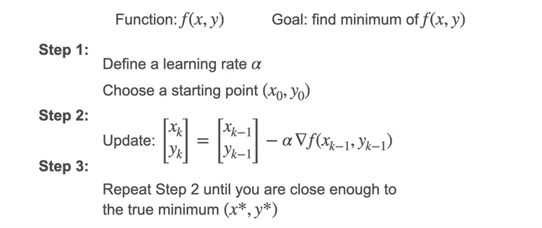
What is Gradient Descent?
Gradient Descent is a technique which we take small steps towards the smaller value and ultimately find the minimum value.
But how do we choose the best possible step so we don’t miss the minimum point? There is a concept called learning rate which decides on the how big the step should be taken so we predict the minimum point in the equation
If the learning rate is big then the steps are too big and you might miss the minimum but if learning rate is small then it takes long to reach the minimum point
What if there are multiple minimum for the equation? The gradient descent may not be successful in finding the minima. The only way is to start from different points to get different minima.