Shilpa Blog

ML Series — Classification with Logistic Regression —A Supervised Machine Learning Algorithm

We know that in supervised machine learning algorithm, we have 2 different types which is regression and classification.

As we are good with linear regression, we are now ready to delve into the next step of supervised machine learning algorithm where we predict the categories.

Classification is used where your output variable y can take on only one of a small handful of possible values instead of any number in an infinite range of numbers. It turns out that linear regression is not a good algorithm for classification problems. Let’s take a look at why and this will lead us into a different algorithm called logistic regression, which is one of the most popular and most widely used learning algorithms today.

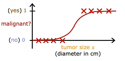
Some examples of classification problems are to determine if email is spam or not, if transaction is fraudulent, if the tumor malignant or benign. The output of these problems is yes or no.

This type of classification problem where there are only two possible outputs is called binary classification.

Where the word binary refers to there being only two possible classes or two possible categories. The one false or 0 is called negative class ( indicates absence) and the true or 1 is a positive class ( indicates presence).

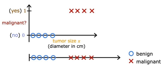
Suppose we represent this in linear regression which is straight line then it looks like this.

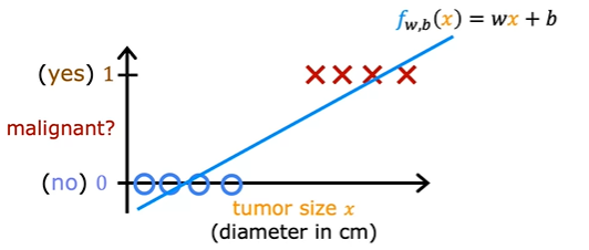
Linear regression predicts not just the values zero and one. But all numbers between zero and one or even less than zero or greater than one. But here we want to predict categories. One thing you could try is to pick a threshold of say 0.5. So that if the model outputs a value below 0.5, then you predict why equal zero or not malignant. And if the model outputs a number equal to or greater than 0.5, then predict Y equals one or malignant. Notice that this threshold value of 0.5 intersects the best fit straight line at this point. So if you draw this vertical line here, everything to the left ends up with a prediction of y equals zero. And everything on the right ends up with the prediction of y equals one. Now, for this particular data set it looks like linear regression could do something reasonable.

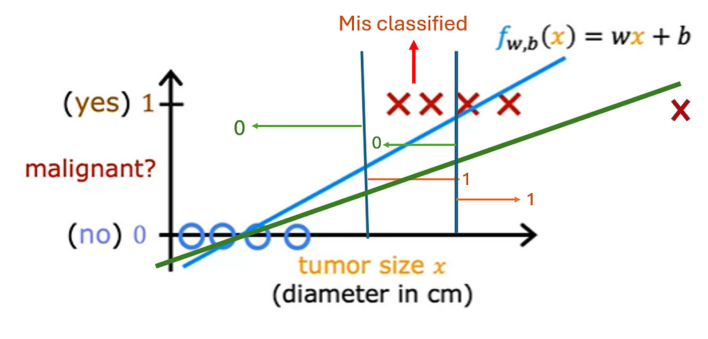
This vertical dividing line that we drew just now still makes sense as the cut off where tumors smaller than this should be classified as zero. And tumors greater than this should be classified as one. But once you’ve added this extra training example on the right. The best fit line for linear regression will shift over like this. And if you continue using the threshold of 0.5, you now notice that everything to the left of this point is predicted at zero non malignant. And everything to the right of this point is predicted to be one or malignant. This isn’t what we want because adding that example way to the right shouldn’t change any of our conclusions about how to classify malignant versus benign tumors. But if you try to do this with linear regression, adding this one example which feels like it shouldn’t be changing anything. It ends up with us learning a much worse function for this classification problem. Clearly, when the tumor is large, we want the algorithm to classify it as malignant. So what we just saw was linear regression causes the best fit line. When we added one more example to the right to shift over. And does the dividing line also called the decision boundary to shift over to the right.

How to solve this problem?

We have a logistic regression we have perfect graph that fits this type of classification.

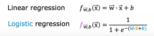
To build out to the logistic regression algorithm, there’s an important mathematical function which is called the Sigmoid function, sometimes also referred to as the logistic function.

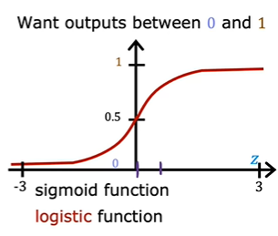
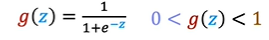
If the z is very large number then the g(z) tends to be closer and closer to 1, and z is large negative number then g(z) tends to be closer to 0. if z =0, then denominator becomes 1 + 1 which is 2 and g(z) would be 0.5.

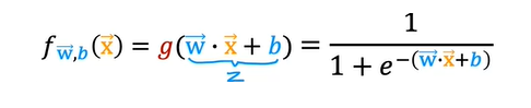
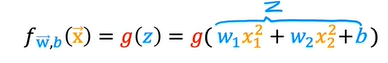
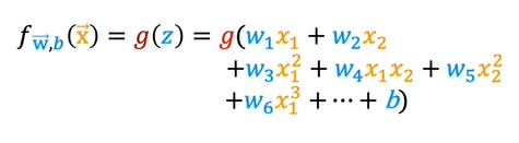
When you take these two equations and put them together, they then give you the logistic regression model f (x), which is equal to g (wx + b). Or equivalently g(z), which is equal to this formula over here. This is the logistic regression model, and what it does is it inputs feature or set of features X and outputs a number between 0 and 1.

We can interpret the logistic regression output as the probability that the class is 1 for certain input.

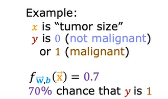
So the sum of probability of y = 0 and probability of y = 1 would be 1

Decision Boundary

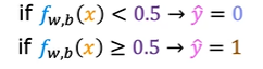
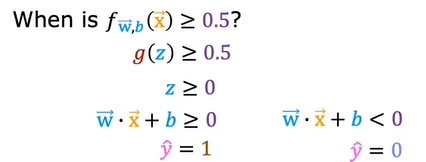
How would we determine if the output is 0 or 1 based on the value of g(z). We take the threshold of 0.5 where f(x) ≥ 0.5 then y^ = 1 and if less than 0.5 then y^ = 0.

Let us take an example of 2 features x1 and x2

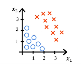
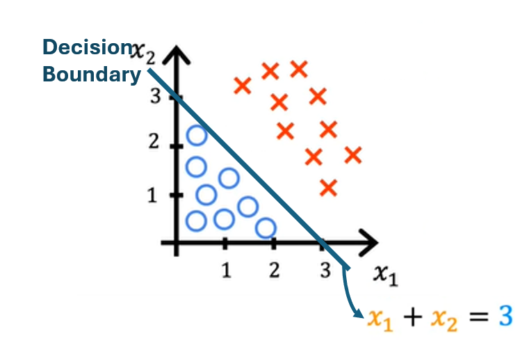
Let us see how logistic regression works here. From the above inference, we got wx + b ≥0 then y^ = 1. This is the decision boundary which is neutral whether the output can be 0 or 1. To find the decision boundary of this line, consider the equation

consider w1 = 1 and w2 = 1 and b = -3. We get the decision boundary when z = wx + b = 0. So we have to determine the line x1 + x2 -3 = 0 which is x1 + x2 = 3. this is the decision boundary line.

What if we have non-linear decision boundary?

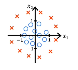
Consider this example.

and now assuming w1 =1, w2 = 1 and b = -1

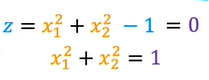
If we have more complex expressions like shown below

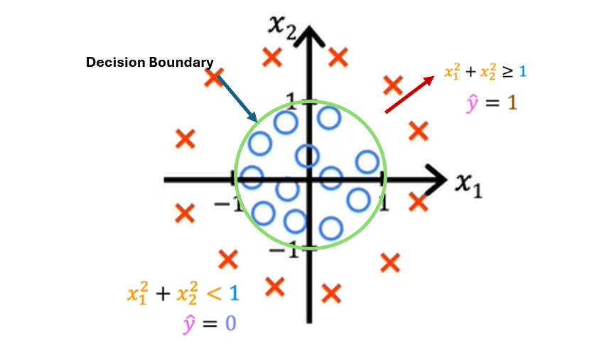
This implementation of logistic regression will predict y equals 1 inside this shape and outside the shape will predict y equals 0. With these polynomial features, you can get very complex decision boundaries. In other words, logistic regression can learn to fit pretty complex data. Although if you were to not include any of these higher-order polynomials, so if the only features you use are x_1, x_2, x_3, and so on, then the decision boundary for logistic regression will always be linear, will always be a straight line.

Cost Function

The cost function gives you a way to measure how well a specific set of parameters fits the training data. Thereby gives you a way to try to choose better parameters.

We have seen the cost function of linear regression as

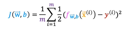
For linear regression, we get the convex cost function and using gradient descent we find the minimum value of J. But if we apply same for logistic regression the cost function would be non-convex and it is not a good fit.

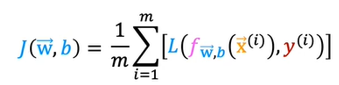
Instead, we have a different cost function so the gradient descent can sure predict the minimum. To create a new cost function, we will consider the expression in the above equation which is after the summation as Loss function.

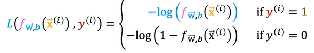
We obtain the cost function by summation of all the loss functions obtained for each training example.

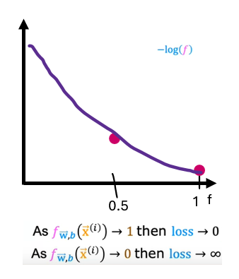
If the algorithm predicts 0.5, then the loss is at this point here, which is a bit higher but not that high. Whereas in contrast, if the algorithm were to have outputs at 0.1 if it thinks that there is only a 10 percent chance of the tumor being malignant but y really is 1. If really is malignant, then the loss is this much higher value over here. When y is equal to 1, the loss function incentivizes or nurtures, or helps push the algorithm to make more accurate predictions because the loss is lowest, when it predicts values close to 1

Let us consider other condition, -log(1-f)

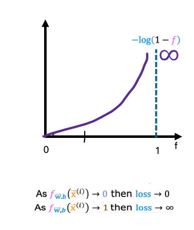
When this function is plotted, it actually looks like this. The range of f is limited to 0 to 1 because logistic regression only outputs values between 0 and 1. In this plot, corresponding to y equals 0, the vertical axis shows the value of the loss for different values of f of x. When f is 0 or very close to 0, the loss is also going to be very small which means that if the true label is 0 and the model’s prediction is very close to 0, well, you nearly got it right so the loss is appropriately very close to 0. The larger the value of f of x gets, the bigger the loss because the prediction is further from the true label 0. In fact, as that prediction approaches 1, the loss actually approaches infinity. Going back to the tumor prediction example just says if the model predicts that the patient’s tumor is almost certain to be malignant, say, 99.9 percent chance of malignancy, that turns out to actually not be malignant, so y equals 0 then we penalize the model with a very high loss. In this case of y equals 0, so this is in the case of y equals 1 on the previous slide, the further the prediction f of x is away from the true value of y, the higher the loss. In fact, if f of x approaches 0, the loss here actually goes really large and in fact approaches infinity. When the true label is 1, the algorithm is strongly incentivized not to predict something too close to 0.

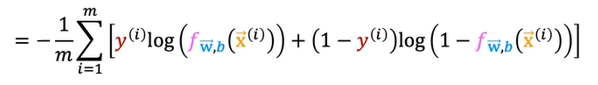
Simplified Cost Function

The above equation can be rewritten as

If yi = 1 then second expression turns out to be 0 and so it is same as the above defined which is log(f). Similarly, yi =0, we get -log(1-f)

Now if we write the cost function from this which is applying the summation we get

This is derived from the statistical function which is maximum likelihood generation

Applying Gradient Descent

From the above, we know that the cost function. If we have to apply gradient descent we use

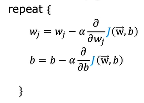
j goes from 1 to n where n is number of training examples

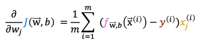
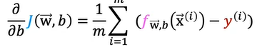
These equations looks similar to that of the linear regression. But the difference is

These 2 are same concepts. We monitor the learning curve to determine if gradient descent converges. We can also apply the vectorized implementation and feature scaling similar to that of linear regression.