ML Series — How can regularization reduce Overfitting of a model?
Overfitting and Underfitting in Linear Regression
Linear Regression and Logistic Regression works well for many tasks but sometimes in an application, the algorithm can run into a problem called overfitting, which can cause it to perform poorly. There are some techniques for reducing this problem. One such technique is Regularization.
Regularization will help you minimize this overfitting problem and get your learning algorithms to work much better.
Let us take an example, predicting the housing prices with linear regression, where you want to predict the price as a function of the size of a house. Suppose we have an input feature x being the size of the house and the value y that you are trying to predict the price of the house. What we do in linear regression is we fit the linear function to the data. If we do that, we get a straight line fit to the data that may be look like this.
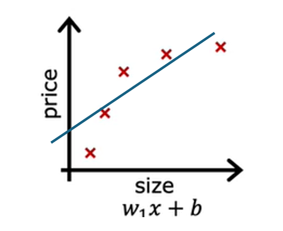
This is not a good model. Looking at the data, it seems to the pretty clear that as the size of the house increases, the housing process flattened out. This algorithm does not fit the training data very well. The technical term for this is the model is underfitting the training data. Another term is the algorithm has high bias.
Checking learning algorithms for bias based on the characteristics is absolutely critical. But the term bias has a second technical meaning as well, which is if the algorithm has underfit the data, meaning that it’s just not even able to fit the training set that well. There’s clear pattern in the training data that the algorithms is just unable to capture. Another way to think of this form of bias is as if the learning algorithm has a very strong preconception, or we say a very strong bias, that the housing prices are going to be a completely linear function of the size despite data to the contrary. This preconception that the data is linear causes it to fit a straight line that fits the data poorly, leading it to underfitted data.
Now, let’s look at a second variation of a model, which is if you insert for a quadratic function at the data with two features, x and x², then when you fit the parameters W1 and W2, you can get a curve that fits the data somewhat better. Maybe it looks like this. Also, if you were to get a new house.
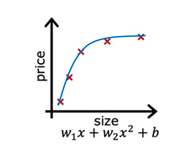
This model would probably do quite well on that new house. If you’re real estate agents, the idea that you want your learning algorithm to do well, even on examples that are not on the training set, that’s called generalization. Technically we say that you want your learning algorithm to generalize well, which means to make good predictions even on brand new examples that it has never seen before. These quadratic models seem to fit the training set not perfectly, but pretty well. I think it would generalize well to new examples.
Now let’s look at the other extreme. What if you were to fit a fourth-order polynomial to the data? You have x, x², x³, and x⁴ all as features. With this fourth for the polynomial, you can actually fit the curve that passes through all five of the training examples exactly. You might get a curve that looks like this.
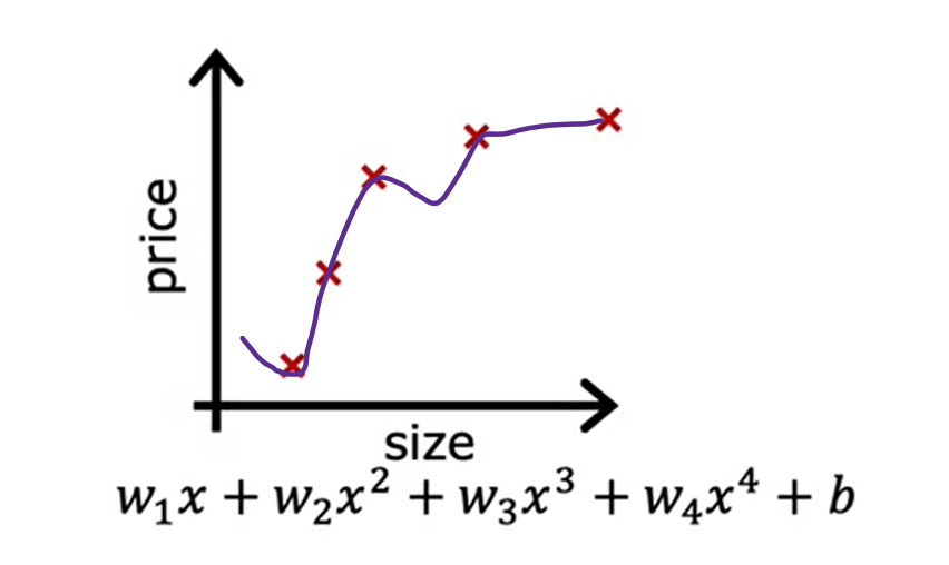
This is extremely good job fitting the training data because it passes through all of the training data perfectly. In fact, you would be able to choose parameters that will result in the cost function being exactly equal to zero because the errors are zero on all five training examples. But this is very wiggly curve, it is going up and down all over the place. The model would predict that this house is cheaper than the houses that are smaller than it. The technical term is that we ll say this model has overfit the data or this model has an overfitting problem because even though it fits the training set very well, it has fit the data almost too well, hence overfit.
In machine learning, many people use terms over-fit and high variance almost interchangeably. The intuition behind overfitting or high variance is that the algorithm is trying veery hard to fit every single training example. If two different machine learning engineers were to fit this fourth-order polynomial model, to just slightly different datasets, they couldn’t end up with totally different predictions or highly variable predictions. That’s why we say the algorithm has high variance. So the model in machine learning is to have neither high bias nor high variance.
In the above examples, the quadratic function is just the right fit.
Overfitting and underfitting in Classification
Overfitting applies to classification as well. Let us take an example of classifying tumor as malignant or benign with 2 features x1 and x2 which is tumor size and age of patient.
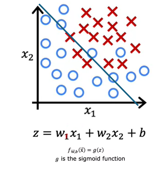
One thing you could do is fit a logistic regression model. g is the sigmoid function and this term here inside is z. If you do that, you end up with straight line as the decision boundary. This is the line where z = 0 that separates the positive and negative examples. But this line does not look like fit the data very well. This is the example of underfitting or of high bias.
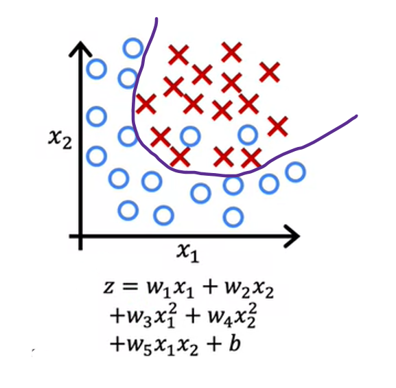
If you were to add to your features these quadratic terms, then z becomes this new term in the middle and the decision boundary, that is where z equals zero can look more like this, more like an ellipse or part of an ellipse. This is a pretty good fit to the data, even though it does not perfectly classify every single training example in the training set. Notice how some of these crosses get classified among the circles. But this model looks pretty good. I’m going to call it just right. It looks like this generalized pretty well to new patients.
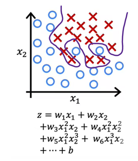
Finally, at the other extreme, if you were to fit a very high-order polynomial with many features like these, then the model may try really hard and contoured or twist itself to find a decision boundary that fits your training data perfectly. Having all these higher-order polynomial features allows the algorithm to choose this really over the complex decision boundary. If the features are tumor size in age, and you’re trying to classify tumors as malignant or benign, then this doesn’t really look like a very good model for making predictions. Once again, this is an instance of overfitting and high variance because its model, despite doing very well on the training set, doesn’t look like it’ll generalize well to new examples.
Now you’ve seen how an algorithm can underfit or have high bias or overfit and have high variance. You may want to know how you can give get a model that is just right.
How to address overfitting?
There are 3 main ways to avoid overfitting of data —
- Get more data which means you can collect more training data
- Selecting and using only a subset of the features. You can continue to fit a high order polynomial or some of the function with lot of features
- Reduce the size of the parameters using regularization by eliminating some features
Cost Function with Regularization to avoid overfitting
In the above example, we saw that if you fit a quadratic function to this data it gives a pretty good fit. But if you fit a very high order polynomial you end up with a curve that over fits the data. Suppose that you had a way to make the parameters W3 and W4 really small say close to 0. So we are effectively nearly cancelling our the effects of the features execute and extra power of 4 and get rid of these 2 terms. We get the fit to the data that is closer to the quadratic function. This is the idea behind regularization.
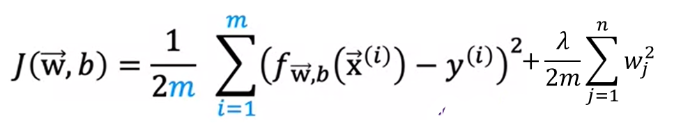
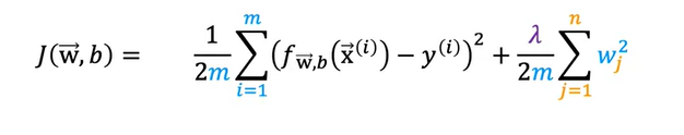
Generally, the way that regularization tends to be implemented is if you have a lot of features, say 100 features, you may not know which are the most important features and which ones to peanlize. So the way regularization is typically implemented is to penalize all of the features by adding a term lambda times the sum from J from 1 to 100. The number of features of wj squared. This value of lambda is called a regularization parameter. Along with this we have 1/2m in the cost function, so we also scale the second parameter with the same 1/2m
It turns out that by scaling both terms the same way it becomes a little bit easier to choose a good value for lambda. And in particular you find that even if your training set size growth, say you find more training examples. So m the training set size is now bigger. The same value of lambda that you’ve picked previously is now also more likely to continue to work if you have this extra scaling by 2m. Also by the way, by convention we’re not going to penalize the parameter b for being large. In practice, it makes very little difference whether you do or not. And some machine learning engineers and actually some learning algorithm implementations will also include lambda over 2m times the b squared term. But this makes very little difference in practice and the more common convention.
So to summarize in this modified cost function, we want to minimize the original cost, which is the mean squared error cost plus additionally, the second term which is called the regularization term. And so this new cost function trades off two goals that you might have. Trying to minimize this first term encourages the algorithm to fit the training data well by minimizing the squared differences of the predictions and the actual values. And try to minimize the second term. The algorithm also tries to keep the parameters wj small, which will tend to reduce overfitting. The value of lambda that you choose, specifies the relative importance or the relative trade off or how you balance between these two goals.
If lambda is low, then the overfitting problem will still exist. If we choose lambda is high, then it make all the weights to be closer to 0 which then equals b which is straight line and it is under fit. So the value of lambda should be not high or not low but just fit.
Regularized Linear Regression
Let us see how gradient descent works with regularized linear regression
We have seen the regularization linear regression as
Now after applying regularization, the gradient descent which is partial derivative with respective to W changes but the partial derivative with respect to b do not change. It looks like this
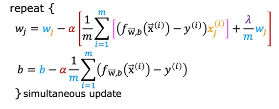
Regularized Logistic Regression
We have seen in the above example, the logistic regression overfitting case with the polynomial expression. We can add the regularization term to the cost function we get by multiplying lambda over 2m
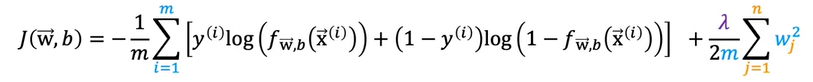
The gradient descent would be as follows on substituting the regularization term and partial derivative on wj
This is similar to linear regression except the function f is the logistic function and not linear function.
Happy Learning!!