Before jumping on to the concept of Maximum Likelihood Estimation which is important in training model in machine learning. Let us understand what point estimation is with respect to statistics. Then we dig into most common point estimation method that’s called Maximum Likelihood Estimation or MLE.
MLE is simple concept. Imagine we have some evidence of something and you wanted to find the scenario that may have led to the evidence so you pick out of all the possible scenarios, the one that created the evidence with highest probability. For Example, there was a game conducted and 3 teams from different states has come. Team A has record of all time win. Team B has record of one time record of won till now. Team C has never won. Who would win the game? Team A is most likely to win the game as the evidence shows they always won. So P(win|Team A) is higher than any other. Similarly, Suppose we have to Estimate the model that would have generated the data.
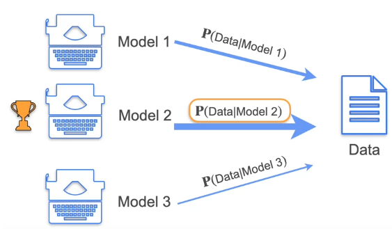
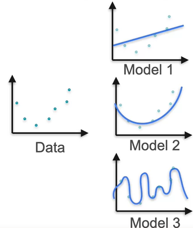
We calculate the probability of Data being generated from Model 1, 2 and 3. The Probability of Data created from Model 2 is higher so Maximum Likelihood of Model 2 generating data is higher. This is the concept of MLE
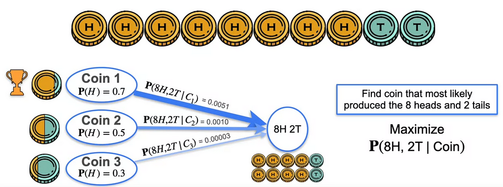
Suppose you have to estimate the outcome with 8Heads, 2 Tails. Coin 1 has the probability of P(H) — The Probability of heads being the outcome is 0.7, For Coin 2 is P(H)=0.5 and for Coin 3 P(H) = 0.3. P(8H, 2T | Coin) is maximum for Coin 1 producing this outcome.
Suppose we have n coins and we have to find the number of the probability that causes k heads. To maximize the function of p which is probability we use logarithm which turns the product of probabilities of each coin to sum.
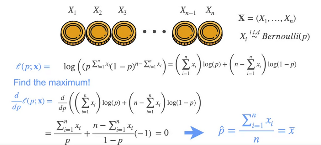
To find the maximum, we find the derivation and it is equal to 0. that would be the mean of the population. So if we have to get K heads then the optimum probability of k heads would be k over n.
Consider the distribution, how will we estimate that the most likelihood of the event happening.
Consider 2 normal distributions with mean and variance as shown below.
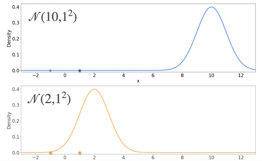
Suppose we have the data points (-1,0) and (1, 0). Which of the above would be most likely generated from these data points?
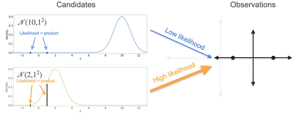
Calculate the heights at -1 and 1.Here the second one has most likely would have been generated from the data points.
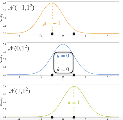
Out of these 3, the possibility for the data points -1 and 1 would be the one with the mean = 0.
The best distribution is the one where the mean of the distribution is the mean of the sample.
What of all of the distributions has same mean but varied variance.
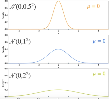
Calculate the variance of each distributions, the first one has 0.5, second one has 1 and third one has 2. The second one is the optimal one.
The best distribution is the one where the variance of the distribution is the variance of the sample.
Mathematical Formulation
Suppose you have n samples X=(X1,X2,…,Xn) from a Gaussian distribution with mean μ and variance σ². This means that Xi∼Normal Distribution (μ,σ²).
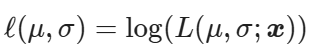
If you want the MLE for μ and σ the first step is to define the likelihood. If both μ and σ are unknown, then the likelihood will be a function of these two parameters. For a realization of X, given by x=(x1,x2,…,xn):
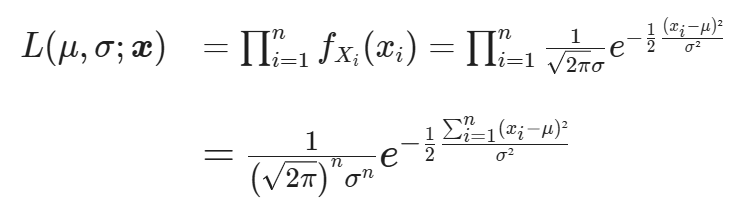
Now all you have to do is find the values of μ and σ that maximize the likelihood L(μ,σ ; x).
You might remember from the calculus course that one way to do this analytically is by taking the derivative of the Likelihood function and equating it to 0. The values of μ and σ that make the derivative zero, are the extreme points. In particular, for this case, they will be maximums.
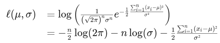
Taking the derivative of the likelihood is a cumbersome procedure, because of all the products involved. However, there is a nice trick you can use to simplify things. Note that the logarithm function is always increasing, so the values that maximize L(μ,σ;x) will also maximize its logarithm. This is the log-likelihood, and it is defined as
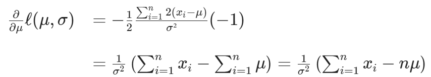
Now to find the MLE for μ and σ, all there is left to do is take the partial derivatives of the log-likelihood, and equate them to zero.
For the partial derivative with respect to μ note that the first two terms do not involve μ, so you get:
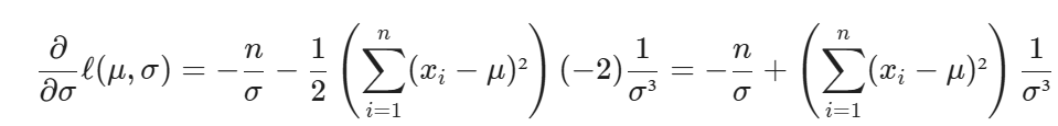
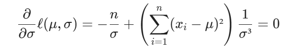
Now partial derivative with respect to σ is
Now equating it to 0
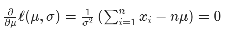
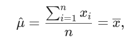
This is nothing but sample mean
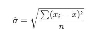
This expression tells you that the MLE for the standard deviation of a Gaussian population is the square root of the average squared difference between each sample and the sample mean. This is same as sample standard deviation except we have 1/(n-1)
MLE For Linear Regression
Consider the following models that would be generated by the data
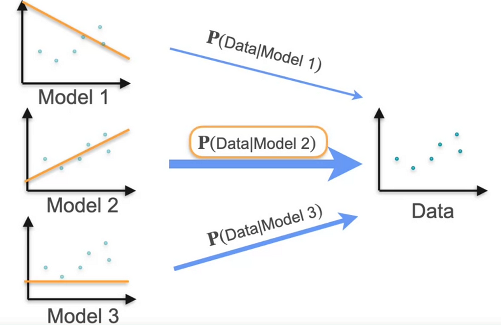
Model 2 is likely to be generated from data.
Suppose we have the best fit line as y = mx + b and let us say there are points that intersect this line and there are other blue points that generated these points.
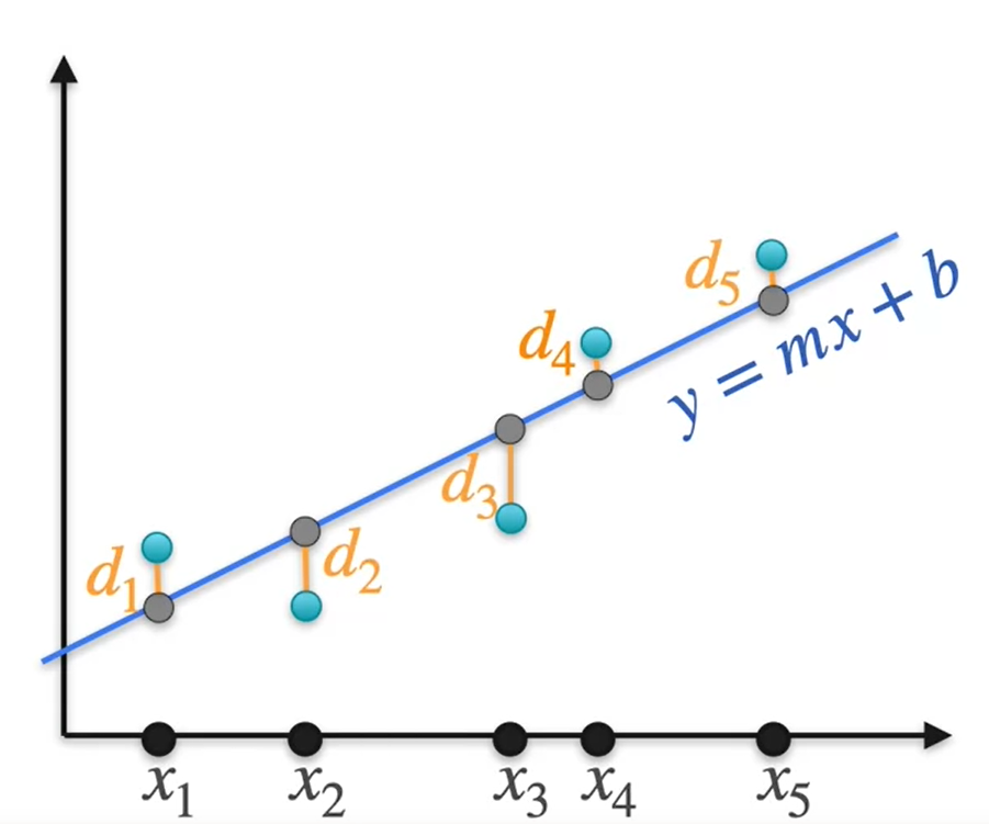
let the points be d1, d2, d3, d4, d5. At each point let us draw the Gaussian distribution
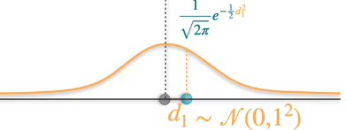
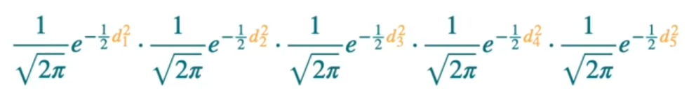
Our data point d1 is not on the best fit line. So the blue point is the original data point and the black point is the point on best fit line corresponding to it. So from the above the Gaussian distribution most likelihood of generating the point d1 on the best fit line is given by the formula
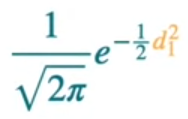
Similarly, we can get the likelihood for other points as well. The product of all the points would be likelihood of generating all points.
When we maximize these, we can eliminate the constants
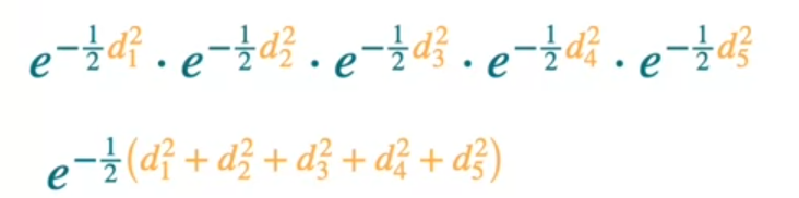
So we know that maximizing something is maximizing the logarithm and also to the 1/2 it would multiply by 2. But as you see we have negative number here that means we have to minimize the sum of squares.
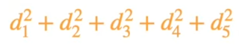
Minimizing the sum of squares is precisely the least square error. That is what exactly linear regression is. That is minimizing the sum of squared distances from the point.
This shows that finding the line that most likely produce a point using maximum likelihood is exactly the same as minimizing the least square error using linear regression
How about polynomial regression?
Suppose we have the data points. We have 3 models and we should know which one is maximum likelihood that is created from the data set.
If you calculate loss of each model, we get Model 3 has the least amount of loss as it follows each data point. But this is little chaotic. So we have to regularize this in order to estimate the maximum likelihood. For this, let us consider the equations of each of these lines.
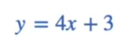
Model-1 equation
Model-2 equation

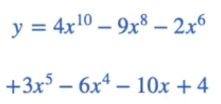
Model-3 equation
Now that we have got the equations, we have to calculate the penalty. The penalty is sum of squares of the coefficients of the expressions. The Model-1 gets 16 and so new loss would be adding the penalty to the loss we calculated. let say loss is 10. The new loss would be 26. For the second model, the sum of coefficients is 20 and the new loss is 22. for the third model, the sum of coefficients is 246 and new loss would be 246.1. So the model 2 is the most likelihood. So what we did here is we modify the loss and we penalize the models that are too complex. In that way, we’re sort of trying to find the simplest model that fits the data well.
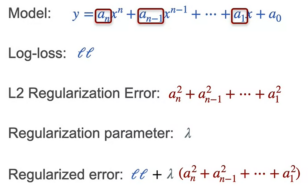
In general, if the model has this equation of a polynomial and the log loss is e.g. LL, then the L_2 regularization error is sum of the squares of the coefficients that are not the last one, that are not the constant one. We’re going to have something called a regularization parameter, because sometimes we don’t want to apply the full penalty, we want to multiply it by a small number in order to not be too drastic here. The regularized error is simply the log loss plus the regularization parameter times the L_2 regularization error.
This helps in reducing overfitting of the model into the data.
Bayesian Statistics

In Bayesian Statistics, the probability changes with the prior belief and the evidences changes the values of posterior values. In the above case, the left hand side is the posterior value which is obtained on multiplying with the prior which is Py and fy. This is nothing but MAP which is Maximum Posterior Estimation.
The main idea behind the Bayesian Statistics is
- Bayesians update prior beliefs
- MAP with uninformative priors is just MLE
- with enough data, MLE and MAP estimates usually converge
- Good for instances when you have limited data or strong prior beliefs
- Wrong priors will lead to wrong conclusions