Probability Distribution is one of the important concept when it comes to analyzing the Discrete and Continuous values of Random values at which the probability of occurrence of an event can be calculated.
- Probability — How is it related to Machine learning?
- Advanced Probability Concepts for Machine Learning
Every one who is aware of probability distribution should be good with few concepts. They are none other than Mean, Median and Mode which are simple yet powerful topic to describe the center of the distribution an d also variance which describes the spread of the distributions.
What is Expected Value?
We know that the mean is the sum of all the values and divide by the total number of items which gives average.
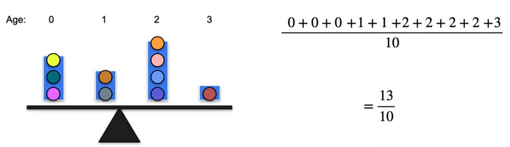
The above shows average age of kids which is nothing but mean. It can also be written as 3 times 0, 2 times 1, 4 times 2 and 1 time 3. If we split them a little bit and see 3/10 which is probability of occurring 0 age multiplied by the weight which is the age.
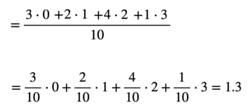
So the Expected value here is 1.3. Here, if you observe 0, 1, 2, 3 are discrete random variables multiplied by its respective probabilities. Let us generalize this for Discrete random variables the expected value is
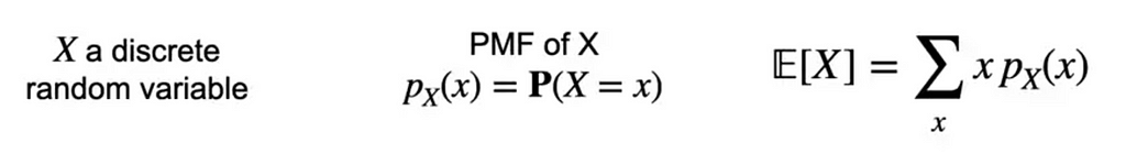
The sum of probabilities should be 1 always
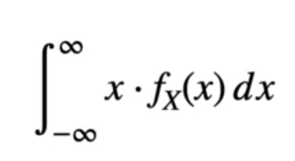
What about Continuous Random variables?
As it is continuous and the values of x can be anything between the intervals. The formula would change a bit using the integration.
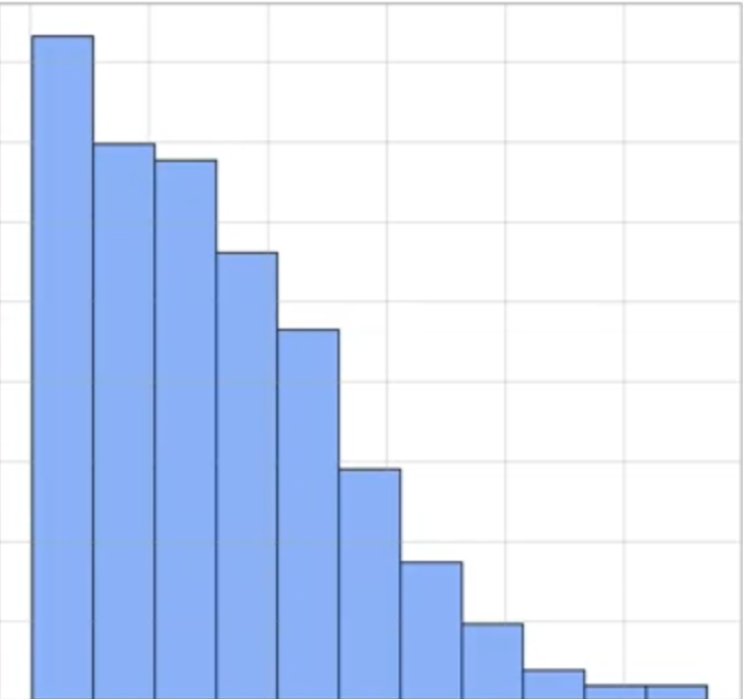
In the probability distribution of continuous variables, the data points are distributed something like this
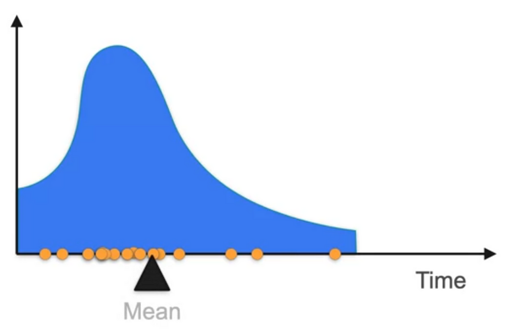
Where the mean is located somewhat at the edge and not at the middle because of the weights that are more on the right side compared to that of left side. Therefore, the mean does not give the exact middle point of the distribution. So what is the solution of Expected value.
In this case, if there is one value that is far above the other and when weighted high, the mean would not give the correct value as it is biased due to the data point that is out of range which is called Outlier.
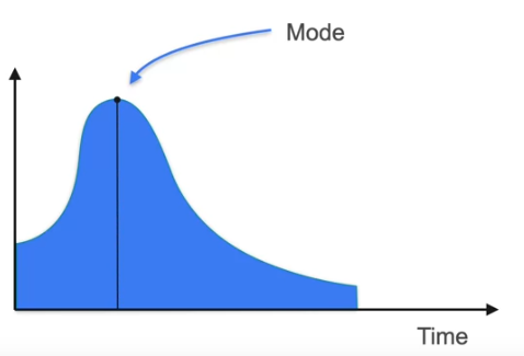
Here the best method to follow is Median or Mode.
Median is the center value where half of data lies to the left and half to the right. Mode is the the value that is most repeated data point.
In normal distribution, which is the symmetric curve, the mean, median and mode are all the same.
Now we have seen the Expected value of the random variables which are the numbers but what if it is function like x³ or x²
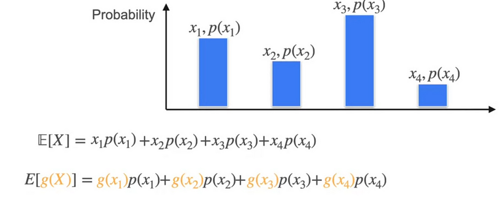
We simply replace the x₁, x₂ with the functions.
E[X] is the linear operated which means if E[aX+b] = aE[X] + b
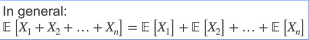
The Expectations value of a sum of n variables is the sum of the expected values.
The Expected values gives some information about the distribution but not all. Two cases the expected value might be same but one can be wide and other can be narrow. So how can we find this. This is defined by how much the distribution is spread. It can be given by Variance.
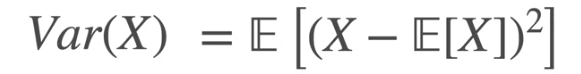
In the above case, if the Expectation is positive for some and negative for other then it gets nulled. So in order to preserve the deviation from the mean we always consider squared value which does not consider if negative or positive.
So for the above expression, we follow the steps
- Find X’s mean
- Find the deviation from that mean for every value of X
- Square those deviations
- Average those squared deviations
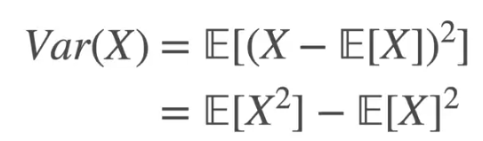
The above expression can also be written using the sum of expectations rules as
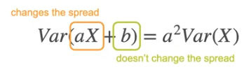
If the variance is multiplied by a constant even the spread increase by that constant. But if the addition is done to the variance it does not have affect
What if we have some units like mm or km. The variance gives the spread in mm² and km² which is different metrics. So we take the square root of variance which is called Standard Deviation
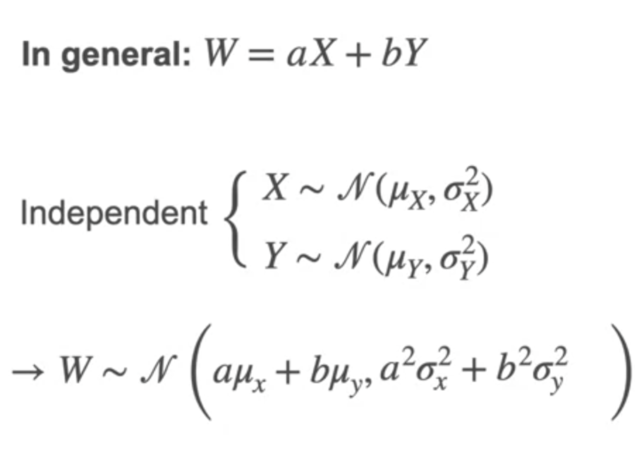
What happens to the Gaussian distribution when added together what happens to the mean and standard deviation and Gaussian distribution. As Mean and Variance has the linear property, the gaussian distribution looks like this
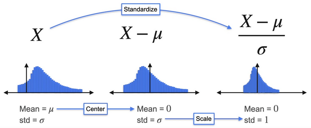
Standardizing distributions
We usually standardize the distribution by subtracting the mean so the distribution is around the 0. What about standard deviation? To standardize the distribution we can divide the X by standard deviation. Remember, here we are using standard deviation and not the variance.
Why do we do Standardization of distributions?
- It is useful for comparability between different datasets
- Simplifies the statistical analysis
- Improves the performance of machine learning models
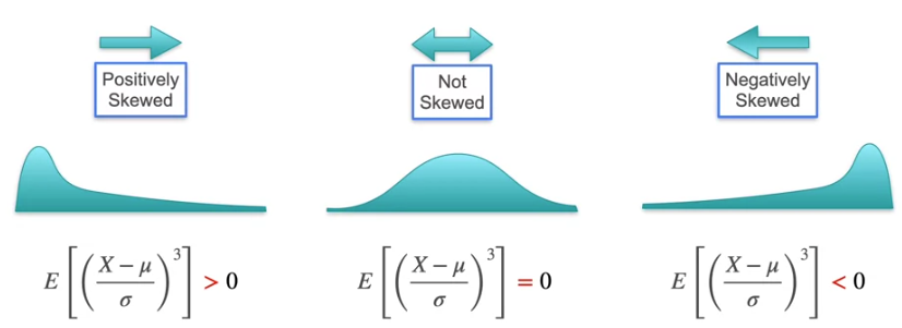
Skewness and Kurtosis
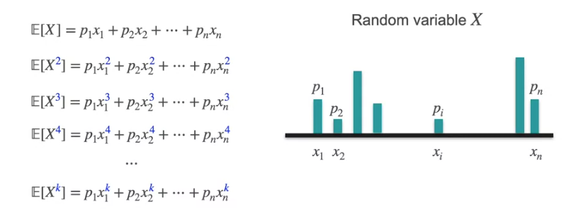
The moments of distribution is X at the first moment and X² at the second moment and X^k at the kth moment
Let us consider the example where we win $100 with the ticket $1 and also you job is Insurance agent where you provide insurance costs $1 and if we repair the car $100. In both the cases, though we gain in first case and loose in other case, the Expected value and Variance is same. But how will we show one is gain and other is loss. This is where the First moment, second moment that we defined earlier is useful.
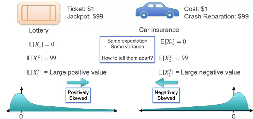
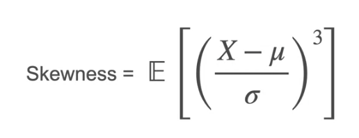
In this example, the 3rd moment shows the difference of skewness which means if it is largely positive which means the distribution is positively skewed and if it largely negative, which means the distribution is negatively skewed.
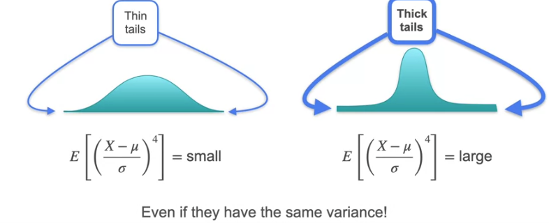
Now that we know the skewness, what if there is normal distribution which is symmetric on both sides. The mean would be 0 and Variance is the spread which is equally spread and it would be 1. The skewness is 0 for symmetric distribution. How to find which has the thick tail and thin tail i.e., the distance between the small amount of tail over the x-axis which is almost negligible in some cases and is high in some cases even if the distribution is symmetric.
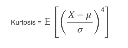
Let us go to the fourth moment which is X⁴. This is Kurtosis
Even if they have same variance the value gives how much
Techniques to Visualize Data
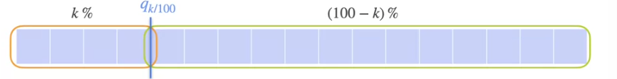
We know that the Median cuts the data points in the half. What if we need some value that cuts the data points into quarter and 3 quarters?
These are called Quantiles.
Box Plot helps to visualize the data based on Quantiles. Q1 is 25% of data, Q2 is 50%, Q3 is 75%. The difference of the value at Q3 to Q1 is the Interquartile Range (IQR)
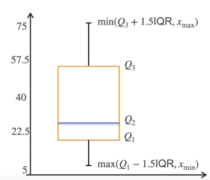
What can you tell from the plot?
- Data is Skewed
- No outliers
- Analyze Dispersion
Kernel Density Estimation
In the continuous Random variable. We know that the distribution is histogram and is not a smooth curve if we take large intervals. This gets to smooth curve if the initial datapoints are more. What should we do if we have limited data points that cannot be plotted for the small intervals. We use Kernel Density Function which gives smooth curve at the points where the density is higher and the value goes down if it is not.
For Example, consider the histogram which is positive and the area is 1 which satisfies the PDF.
In Kernel Density Estimation, we draw the observations along the X — axis
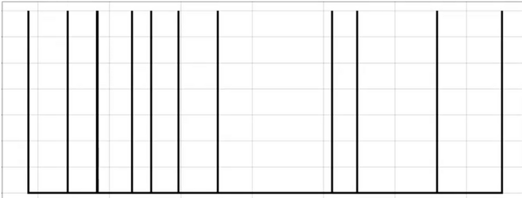
Draw the Gaussian centered at each observation. This is called Kernel
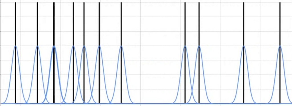
Now multiply everything by 1/n and sum all the blue curves.
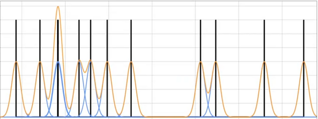
This is for only few points but if we use the larger data set. It looks like a smooth curve. This is how we approximate PDF based on distribution
In the regression models, most of them assume the data is normally distributed. But how do we know it is normally distributed. For this we use QQ plots ( Quantile-Quantile).
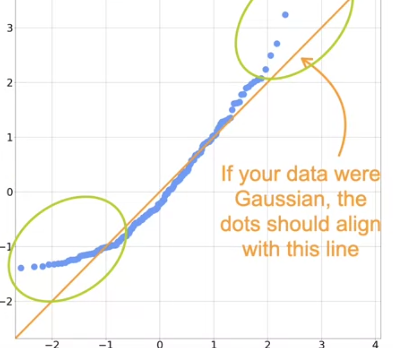
- We standardize the data
- Compute the quantiles
- Compare to Gaussian quantiles
This says if the data is Gaussian distribution or not based on the dots that align with the line
Multiple Variables
To calculate the probabilities of more than 1 variables we use joint distribution
For Discrete random variables, this is simple as it is the product of the 2 probabilities
For Continuous Random Variables,
we plot the variables, X and Y on 2 axis with 2 variables. The mean would be E(X) and Variance is E[X²]-E[X]². Calculate this for both X and Y
What if we wanted to calculate the Distribution of one variable ignoring the other variable. This is called Marginal Distribution. This is calculated by adding the probabilities of each value of X.
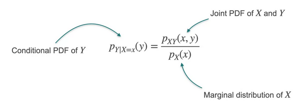
Condition Distribution of the 2 variables where one value of the variable is known would be
What if we have to capture relation between two variables. We want to know how 2 random variables are related. There are 2 important concepts, Correlation and Covariance.
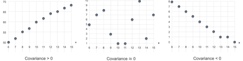
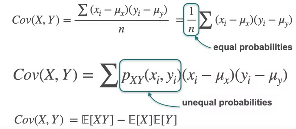
This diagram defines the relation between variables using Covariance. Plot the mean as the 0 of X and Y axis.
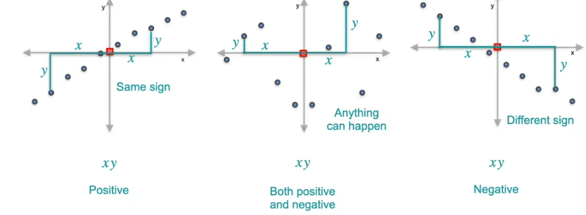
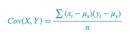
This covariance is calculated by center the data and then you take the average of all these products. This covariance works for the equal probabilities. What if we have unequal probabilities for each case.
Consider the game below
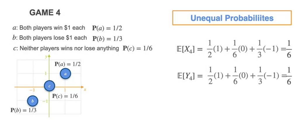
The E[X] and E[Y] are same for both. The variance is given by
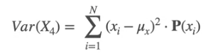
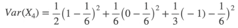
Same for Var(Y)
So the variance would be 0.806. which means X changes positively with Y
Covariance Matrix
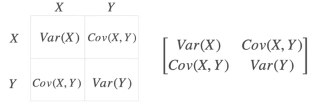
Same can be expanded for multiple variables
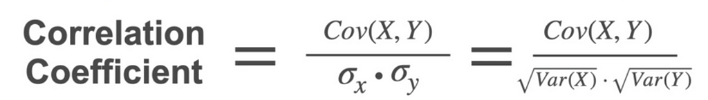
Correlation Coefficient
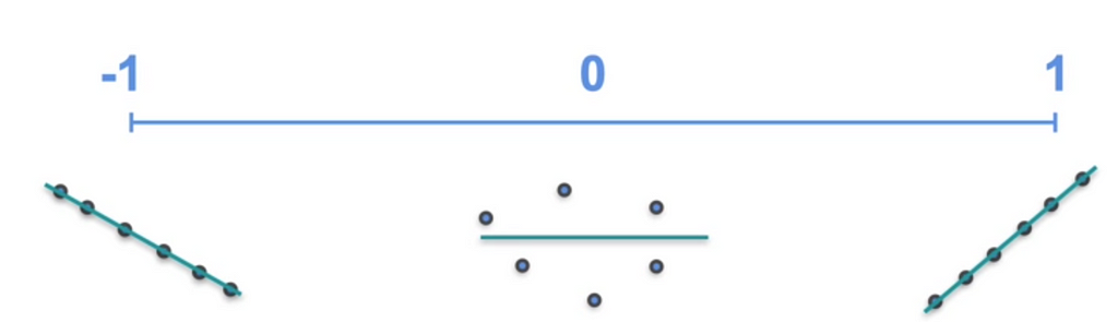
From the covariance, if there are 2 variables X and Y, if the covariance is positive we know that X and Y increases together. Negative says the X and Y decreases together. But how strong is the relation ship. It does not say that. For this we need Correlation Coefficient. The value varies from -1 to 1
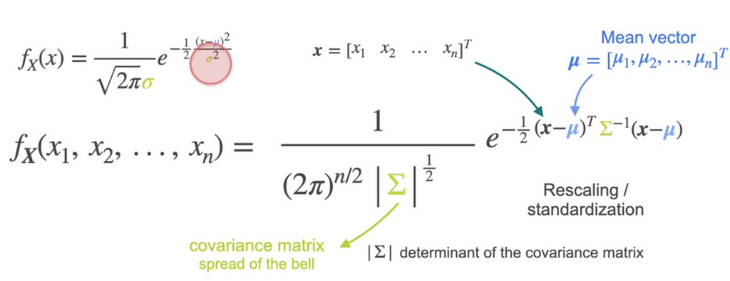
Multivariate Gaussian Distribution
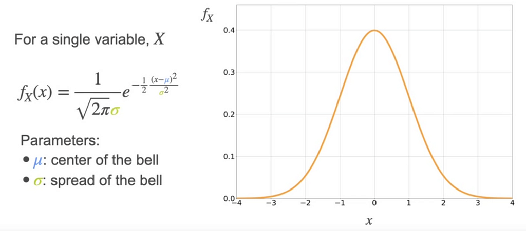
We know that for a single variable, the gaussian distribution is
What if we have multiple variables? Consider 2 variable W and H. If W and H are independent then it is product of fh and fw which gives
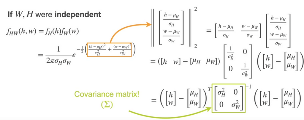
This can be written as
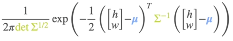
where sigma is Covariance matrix
Happy Learning!
References : DeepLearning.ai